From 50% to 90%+ Forecast Accuracy: What Changes With an AI Layer
Industry research puts forecast accuracy for intermittent demand items at 50-70%. And 70-90% of a typical service parts catalog is intermittent demand - zero usage for months, then unpredictable spikes.
For most service parts organizations, this accuracy range is a familiar frustration. Planning teams invest significant effort in parameter tuning, demand classification, segmentation analysis, and planner-driven overrides. Research from the International Journal of Forecasting (2024) found that planner overrides improve accuracy only about 50% of the time - with upward adjustments actually worsening forecasts more often than not.
The needle moves a few points in either direction. But the fundamental performance level persists.
The instinct is to question the forecasting model. Are we using the right algorithm? Should we switch vendors? Do we need more sophisticated statistical methods?
In most cases, the model isn't the problem. The input is.
The Input Quality Problem
Consider what happens inside an SPM system when it generates a forecast:
- Historical shipment data is loaded (shipments as a proxy for demand)
- Statistical models detect patterns (trend, seasonality, intermittency)
- Install base data adds population-driven demand signals
- Planners apply manual overrides based on domain knowledge
- The resulting forecast feeds inventory optimization
Each step works correctly within its scope. The statistical models are mathematically sound - whether Croston's method, bootstrapping, or reliability-based forecasts for intermittent demand. The optimization logic is rigorous. The planners are experienced.
But the entire process operates within a constrained input set. The demand signal entering the system represents a fraction of the information that drives parts demand. And for intermittent demand items - which characterize most service parts catalogs - the sparse historical signal makes the input quality problem even more acute. When a part sees demand twice in six months, statistical models have almost nothing to work with. The signals that predict the next occurrence (a quality trend, a lifecycle shift, a field-reported failure pattern) sit in adjacent systems the planner can see but the SPM can't.
When a semiconductor manufacturer's quality system detects a component entering early-life failure mode, that signal predicts a demand surge for replacement parts weeks before the historical pattern shows it. When a major customer's CRM records show forward bookings for 200 new units, that signal predicts a future install base (and parts demand) increase that the install base file won't reflect for months. When field technicians document a recurring seal failure in humid climates, that pattern predicts geographic demand concentration that the statistical model can't detect from historical shipments alone.
These signals exist in the enterprise. They're specific, timely, and demand-relevant. They're invisible to the planning system.
The forecast accuracy ceiling at ~60% isn't a model limitation. It's a signal limitation.
What Changes With an AI Operating Layer
An AI operating layer addresses the input quality problem directly. Rather than replacing the forecasting model, it expands the demand signal feeding it.
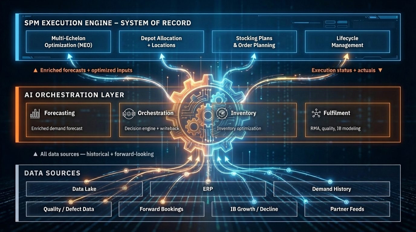
Here's what the architecture looks like in practice:
Signal Aggregation: The AI layer connects to enterprise systems that generate demand-relevant intelligence - quality/MES systems, CRM, field service management, IoT platforms, dealer portals, warranty systems. It ingests signals continuously, not in batch windows.
Pattern Recognition: Machine learning models identify demand-relevant patterns in the aggregated signal - correlations between quality events and parts demand, leading indicators from install base changes, geographic and seasonal patterns that span multiple data sources.
Signal Translation: The AI layer translates these patterns into demand signal enrichments that the SPM system can consume. The SPM doesn't need to change how it processes demand input. It receives a richer, more complete demand signal.
Class-Level Learning: For the 70-90% of parts with sparse demand history, the AI layer learns from the broader part family, equipment class, and failure mode rather than treating each part number in isolation. When a part has moved 3 units in the last year, statistical methods have almost nothing to work with. Class-level learning uses the behavior of related parts to build a prediction that individual data refines over time.
Continuous Learning: As actual demand materializes, the AI layer compares its enriched signal against outcomes and refines its models. New patterns are detected. Stale patterns are deprecated. The signal quality improves with every cycle.
The Impact in Numbers
The accuracy improvement isn't achieved by building a better statistical forecasting model. It's achieved by fundamentally expanding what the forecasting model sees.
Consider the signal gap:
| What SPM Sees | What Drives Demand | Result |
|---|---|---|
| Historical shipments (lagging proxy for demand) | Failure events and quality trends | SPM treats quality-driven demand spikes as statistical noise |
| Basic install base (updated quarterly) | Real-time install base transitions, forward bookings showing fleet changes months ahead | SPM can't see demand shifts until they've already hit |
| Aggregated part-level data | Component-level failures that cross multiple products; manufacturer lot-specific defect rates | Same part number, different behavior - SPM can't distinguish |
| Point-in-time snapshot | 15+ years of lifecycle patterns: compute transitions, product family evolution | SPM batch windows can't process that depth of historical data |
| None | Field technician notes, regional usage patterns, environmental factors | Intelligence locked in people's heads and adjacent systems |
Each additional signal source doesn't replace what the SPM does. It reduces the uncertainty that the SPM operates within. The wider the signal, the bigger the results.
In enterprise deployments, this shows up as specific, measurable outcomes:
- A semiconductor equipment manufacturer reduced 4-week forecast error from 17-18% to under 3% on $50M+ quarterly spend, generating $2M+ in annual savings
- Across deployments, demand forecasting achieves ≤8% MAPE on A-class SKUs and ≤12% on B/C-class items
- Inventory reductions of 15-20% in value and carrying costs
- Stockout reductions of 40% or more
- Planning cycles 80% faster
Not by replacing the optimization engine, but by fixing its input.
Downstream Effects
Forecast accuracy improvement isn't the end goal. It's the enabler for a cascade of operational improvements:
Reduced Expedited Shipments: APQC benchmarks show top-performing organizations spend 3% of total logistics costs on expedited shipping, while bottom performers spend 10% or more - over three times as much. When demand is anticipated rather than reacted to, the right inventory is at the right location before the need arises. For a $2B revenue company, moving from bottom to top quartile on expedited shipping alone represents ~$3.4M in annual savings.
Lower Inventory Investment: Counter-intuitively, higher forecast accuracy enables lower total inventory. SPM vendors themselves claim 20-35% inventory reductions (verified in public case studies from leading platforms). When you trust the forecast, you don't need as much safety stock buffer. Slow-moving items that tie up warehouse space and capital get right-sized based on actual demand intelligence, not conservative min/max policies set years ago. With excess and obsolete inventory typically representing 15-20% of manufacturer inventory, even modest accuracy improvements yield significant carrying cost reductions.
Fewer Stockouts: The tail SKUs that historically caused surprise stockouts - because they weren't being systematically planned - now receive full analytical attention. The AI layer models the complete catalog, eliminating the planning coverage gap.
Planner Productivity: When the forecast is more accurate, override rates drop. Planners spend less time compensating for system gaps and more time on strategic work: vendor negotiations, lifecycle planning, network optimization. And when routine inbox queries - parts availability, order status, "where's my part?" - are auto-resolved (40%+ resolution rates in enterprise deployments, saving 300+ hours per week), planner capacity recovers significantly.
Fill Rate Achievement: The industry average fill rate is 85-92%. Best-in-class organizations achieve 95-98%+. The gap between average and best-in-class represents millions in service contract penalties, customer dissatisfaction, and competitive disadvantage. Better signal means the right inventory position across every echelon - central warehouse, regional depot, van stock - not just at the aggregate level.
First-Time Fix Rate: The industry average first-time fix rate is 75%. Aberdeen Group research shows parts availability is the leading cause of failed first visits 51% of the time - more than technician skills (25%) or insufficient time (13%). Each failed fix requires an average of 1.6 additional dispatches at $200-300 per truck roll. In one enterprise deployment, AI-driven parts prediction pushed FTFR from 75-80% to 88%, saving approximately 30,000 unnecessary truck rolls. Better demand anticipation means the tech has the part when they arrive - even for a 2 AM equipment failure under an SLA.
Lifecycle Intelligence: Supersessions, end-of-life transitions, and repair/return flows are anticipated rather than discovered after the fact. When a part is being superseded, the demand transfer is modeled proactively. When a product line approaches end-of-warranty, the service demand surge is in the forecast before it hits.
The Implementation Path
The accuracy improvement doesn't happen overnight. It follows a predictable progression:
Weeks 1-2: Discovery and baseline. Forward-deployed engineers embed with the planning team, map the signal landscape, and establish current accuracy metrics.
Weeks 3-4: Initial signal integration. The highest-value signal sources (typically quality data and install base lifecycle) are connected first. Initial accuracy improvement is measurable.
Weeks 5-8: Expanded signal fusion and closed-loop feedback. Additional signal sources are integrated. The AI layer begins learning from forecast-vs-actual comparisons. Accuracy improvements compound.
Month 3+: Continuous optimization. New signals are connected as they become available. Models improve with each cycle. The accuracy trajectory continues upward.
The key architectural principle: the SPM system doesn't change. It continues doing what it does well - optimization math. The AI layer improves what it sees - the demand signal. Better input produces better output. That's not a technology revolution. It's applied common sense at enterprise scale.
More in This Series
This article is part of a three-part series on AI operating layers for service parts management:
- The Four Structural Gaps in Modern SPM Systems explores the architectural limitations that create the forecast accuracy ceiling in the first place.
- Why Your SPM Needs an AI Operating Layer lays out the combined architecture and how it complements your existing planning system.
Bruviti builds AI operating layers for service supply chains. We'd love the opportunity to show you what changes when your planning system finally sees the full picture.